Creating an Input-Free Calculator (Without Inputs) #
In this guide, we’ll show you how to create a calculator that does not require any user inputs. Instead, it displays data directly from a connected Google Sheet each time the page is loaded, ensuring the information is always up-to-date.
This is ideal for scenarios where you want to present data without user interaction, like dashboards or reports.
Step-by-Step Guide #
Step 1: Set Up the Calculator as Input-Free #
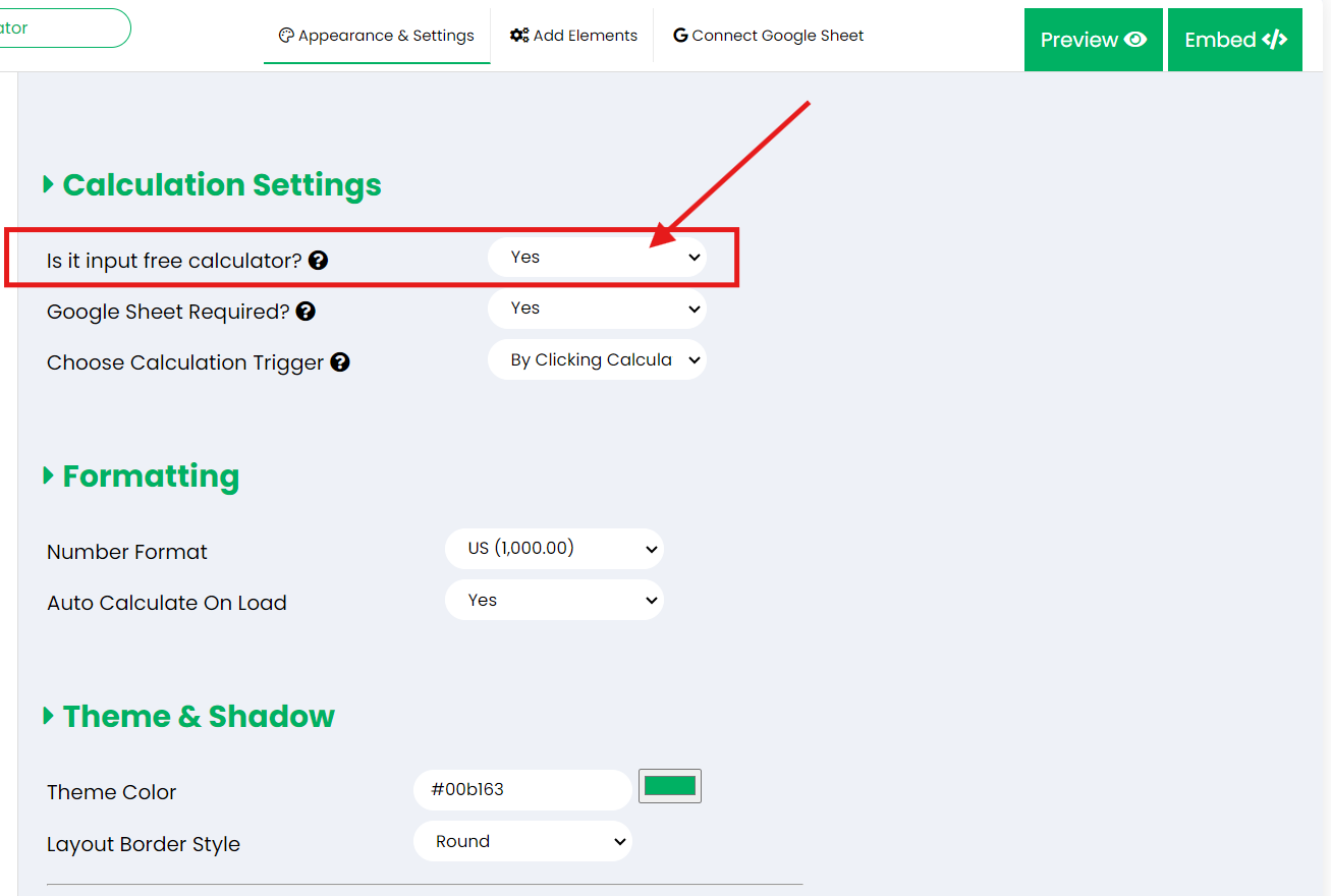
Go to Appearance & Settings > Calculation Settings > Is it input free calculator? and set it to Yes to turn off the requirement for inputs. This will disable the input area in the calculator builder, allowing you to create a display-only calculator.
Step 2: Connect Your Google Sheet to the Calculator #
In the ES Calculator Builder dashboard, create a new calculator.
- Change the sharing settings of your Google Sheet to “Anyone can edit” temporarily.
- Create a new tab in your Google Sheet named “sgsc-link”. The calculator will read output data from this tab. You will need to link outputs from other tabs in the Google Sheet to this “sgsc-link” tab. Use columns C1:Z1000 for results, while columns A:B remain reserved for input-related data even though they are not used in this scenario.
- Go to the calculator builder, click on Connect Google Sheet, enter your Google Sheet URL, and click the “Connect” button.
- Keeping Google Sheet Private: Once the sheet is successfully connected, you can revert the sharing settings to private. To keep it private while allowing the calculator to function, add the following ES Builder account as an editor in your Google Sheet:
embedsheets@googlegroups.com
Step 3: Add Result Elements #
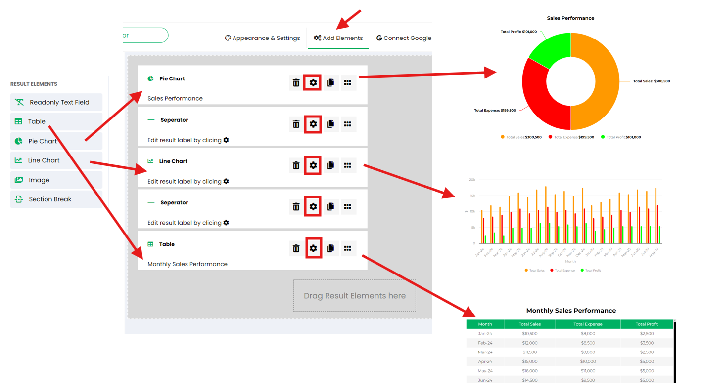
Now that the input area is disabled, you can focus on displaying data from the Google Sheet using various result elements:
- Drag and drop a Table element to display data in a tabular format, such as a summary or detailed view of your data.
- Add a Donut Chart to visually represent proportions or categories from the Google Sheet.
- Include a Line Chart to show trends or data changes over time, using dynamic data from the sheet.
For each of these result elements, link the elements to the relevant cells or data ranges in your Google Sheet to ensure accurate data display.
Step 4: Use a Sample Google Sheet #
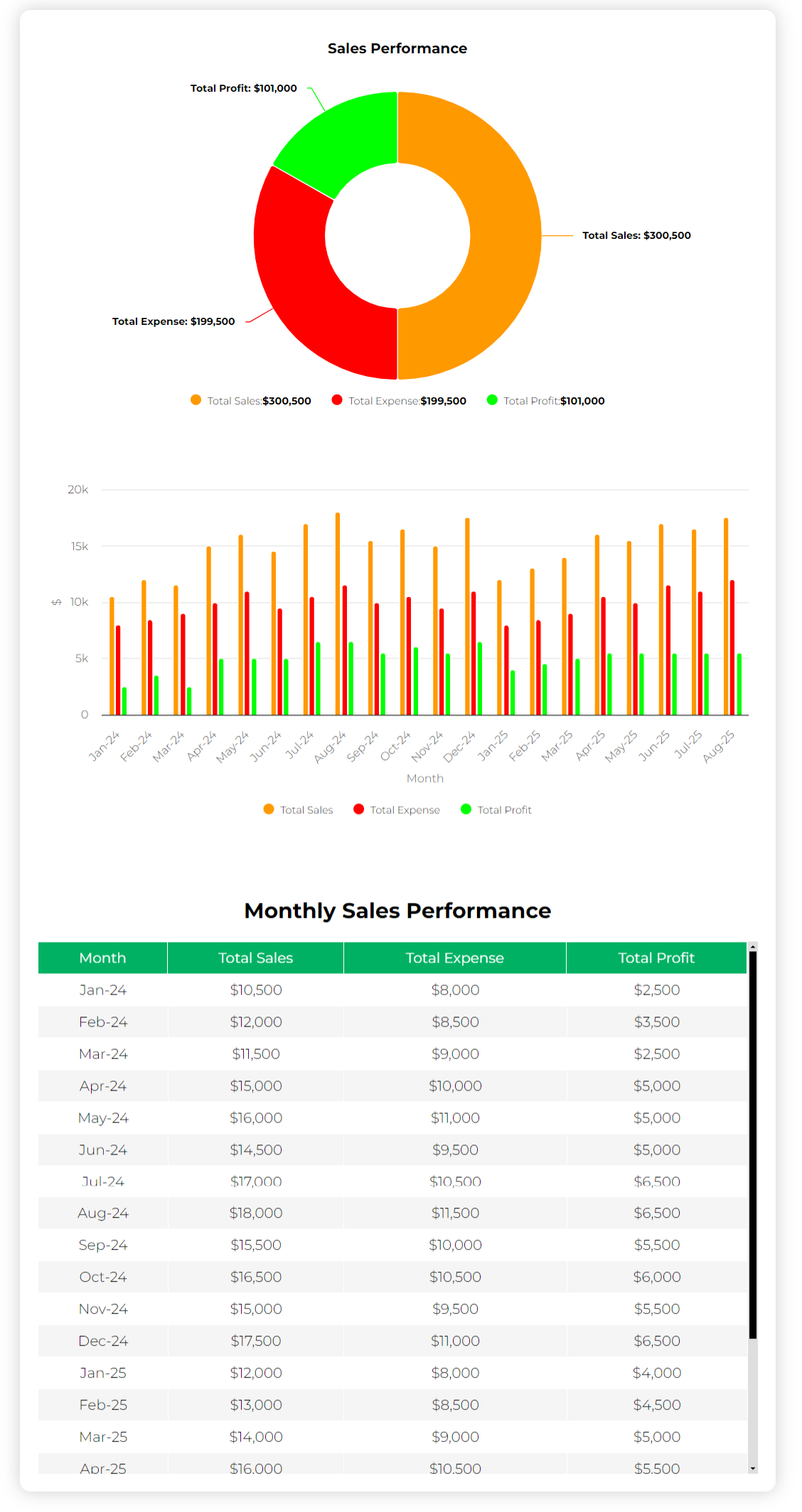
We’ll use a Google Sheet for displaying Monthly Sales Performance as an example to create an input-free calculator that displays data in a table, a donut chart, and a column chart:
https://docs.google.com/spreadsheets/d/18NmgtcsxC1qdn7yyUksfQncltfIGu0n3Y0F_G64HN2k/
The data includes the following:
- Total Sales: Monthly sales data.
- Total Expense: Monthly expense data.
- Total Profit: Monthly profit data.
- Totals: Row 22 in the Google Sheet shows total values for Total Sales, Total Expense, and Total Profit. This row will power the donut chart.
Adding Donut Chart #
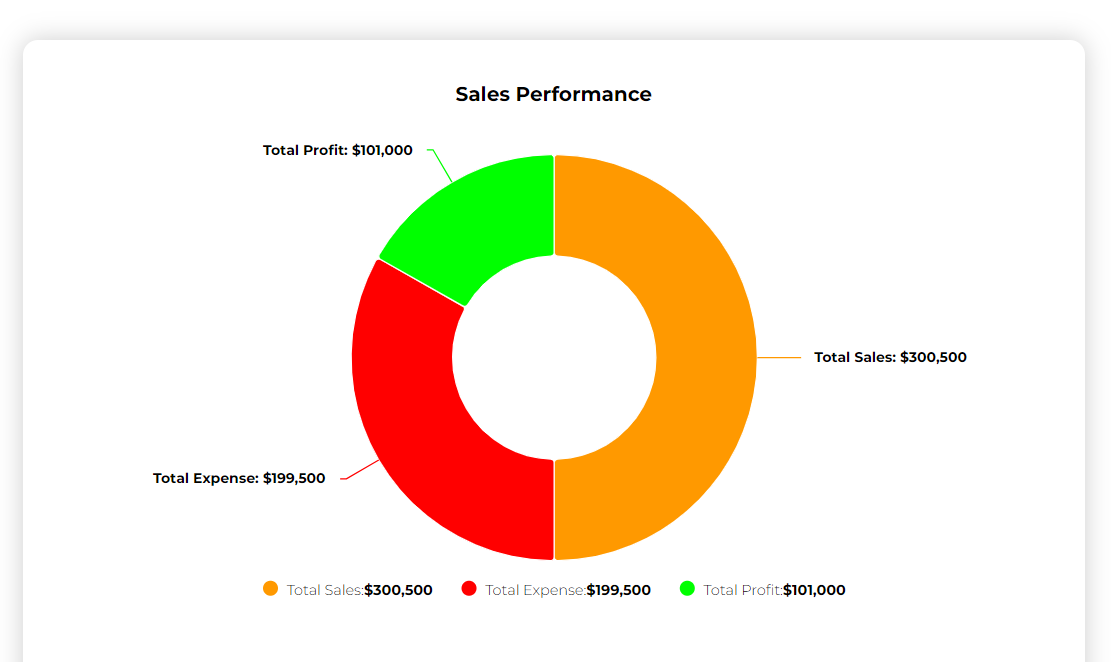
We will add a donut chart for data in the range G3:H5 that displays the total of all months. The configuration is explained in the images below.
In this example, we used specific color codes for the Donut Chart to differentiate between Total Sales, Total Expense, and Total Profit. The color codes used are:To customize the chart with your desired colors, you can obtain color codes using online tools like HTML Color Codes. These tools allow you to select a color visually and provide you with the corresponding hex code, which you can use in your calculator for consistent branding and presentation.
- Total Sales: Orange (#ff9900)
- Total Expense: Red (#ff0000)
- Total Profit: Green (#00ff00)
Adding Column Chart #
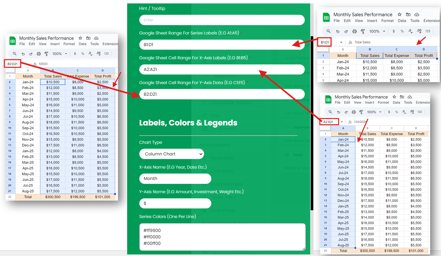
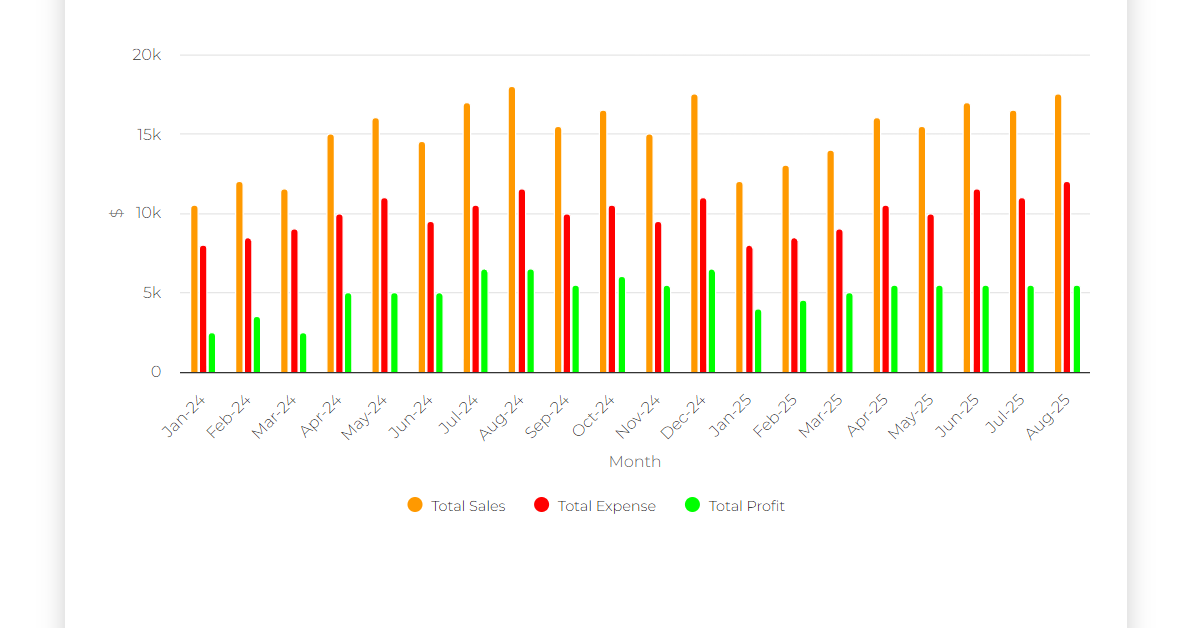
We will add a column chart for data in the range A1:D21 that displays values for each month. The configuration is explained in the images below.
You can use the column stacking option to stack columns in your chart for better data comparison. Additionally, you can switch to a line chart by selecting the desired option from the “Chart Type” dropdown menu.
Adding Table #
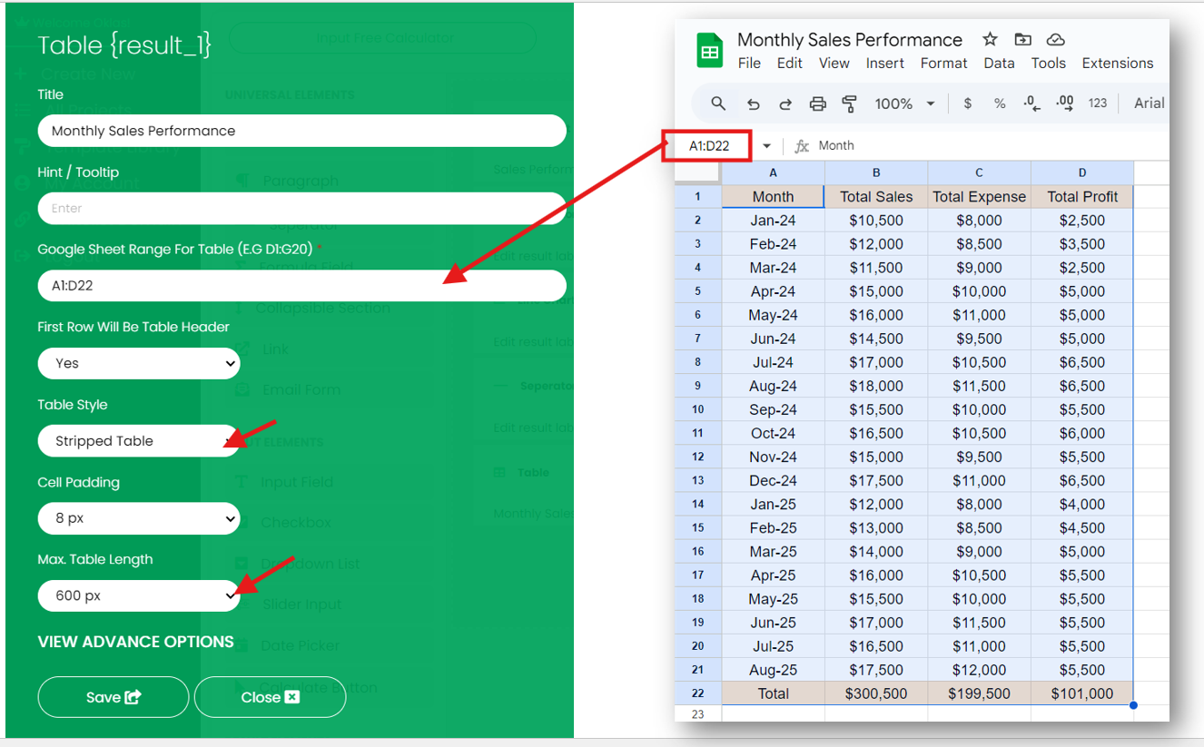
We will also add a table for data in the range A1:D21 that displays values for each month in tabular form. The configuration is explained in the images below.
You can enable / disable scrollbar for lengthy tables using “Max. Table Length” dropdown in table configuration.
Step 5: Customize Appearance and Settings #
Go to the Appearance & Settings tab to adjust layout of your calculator like setting width, shadow etc.
For more details on adjusting calculator settings, visit the Appearance and Settings documentation.
Step 6: Preview and Publish Your Calculator #
Use the preview option to test your calculator. Ensure that the table, donut chart, and column chart display data correctly from the Google Sheet. Adjust the setup if needed for a better user experience.
Once satisfied with the setup, click Embed to generate the embed code. Copy this code and paste it into an HTML block on your website where you want the input-free calculator to appear.
Summary #
By following these steps, you can create an input-free calculator that displays real-time data directly from a Google Sheet. This method is ideal for presenting up-to-date information, such as reports, statistics, or data summaries, without requiring any user interaction. You can use various result elements like tables and charts to visualize the data, making your calculator both informative and visually appealing.
Feel free to explore different data display options and reach out if you encounter any issues while setting up your input-free calculator!
